Continual Learning

Dataset

The full dataset can be downloaded from here: http://clevrer.csail.mit.edu.

VAE

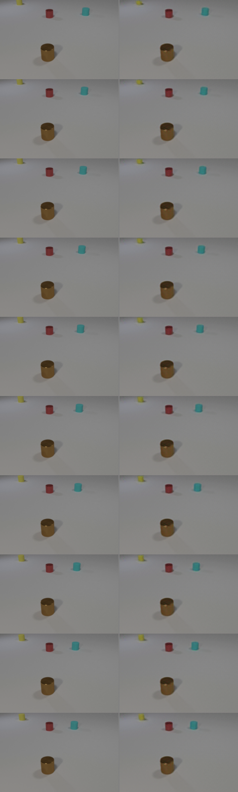
Instead of working with high-resolution pixel space, I trained VAE to represent the frames in a lower dimensional latent space and make the training faster, more efficient and cheaper. After training it for ~300 epochs, the reconstructed frames from the test set latents are shown below. The ones on the left are ground truth test frames and the ones on the right are reconstructed by the decoder.

Optical Flow Model

To obtain ground truth optical flows for supervising the flow head, we can use a pre-trained optical flow model such as RAFT[1], FlowFormer[2], SEA-RAFT[3] or WAFT[4] and precompute the flow fields between each consecutive frame offline.

In this system, I am using RAFT.

Test-Time Training (TTT)

Assuming we choose approach 3, we can utilize the flow predictor head during test-time training. After training the 3 heads jointly, we can continue updating the flow predictor for each video during inference and reset it back to its pre-trained version for each new video.

Loss Functions

VAE

• Reconstruction loss: Pixel-wise L1 loss between the frames decoded from the latents and the actual frames.
• Perceptual loss: L1 loss between the feature maps of the predicted frame and the feature maps of the ground truth frame that are extracted from a pretrained DINOv2 model. It’s internal features respond to edges, textures, shapes, and structure, not individual pixel values. This loss can help us to force VAE decoder to reconstruct the frames that look structurally similar to the target frames.
• KL divergence: Forces the latents to follow a standard gaussian distribution to ensure standardized latent space and make things easier for the temporal model.

Temporal Model

• Latent prediction loss: L1 loss between the predicted next latent and actual next latent.
• Flow loss: The euclidian distance between the predicted optical flow and the actual optical flow.
• Occlusion mask loss: Binary cross entropy-loss between the predicted occlusion mask and forward-backward consistency occlusion mask that is computed from optical flows.
• Warped latent loss: L1 loss between the frame decoded from the warped latent (before residual correction) and the actual next frame.
• Residual loss: L1 loss between the predicted residual and the actual residual
• Collision loss: Focal loss between the predicted collision probability and ground truth binary value that tells us whether collision happened in the specific time frame. The reason why focal loss is used instead of binary-cross entropy is because collisions are rare.
• Uncertainty weigthing: This is a multi-task learning approach. In other words, there are multiple distinct loss functions. Instead of assigning a weight to each loss function manually, we use a different method that automatically adjusts the weights assigned to these loss functions. With this mechanism, these weights can be seen as learnable parameters just like the model weights since the optimizer updates them every step via backpropagation. For small losses, for instance, the system learns to assigns a higher weight while it learns to assign smaller weights for high losses.

Test-Time Training

• Frame reconstruction loss: At each step k, warp frame t using the flow predictor’s output and compare the warped result against the actual frame t+1 with L1 loss.

Evaluation Metrics

• PSNR
• SSIM
• tLPIPS
• IoU of objects over time
• Collision correctness
• Subject consistency
• Background consistency
• Motion smoothness

Training

Phase 1: Train 2D VAE (~50-200 epochs)
Phase 2: Train temporal (~50-100 epochs)
Phase 3: Joint fine-tune (~20-50 epochs)

Precompute Optical Flows

./run_precompute.sh

Train 2D VAE

./run_train_vae.sh

Train Temporal Model

./run_train_temporal

Joint Fine-Tune

./run_joint

Inference

python inference.py \
    --vae_checkpoint checkpoints/vae_epoch0200.pt \
    --temporal_checkpoint checkpoints/temporal_epoch0005.pt \
    --video_folders video_test/video_15000-16000 \
    --img_h 128 --img_w 128 \
    --num_input_frames 20 \
    --num_pred_frames 12 \
    --ttt --ttt_steps 10 \
    --output_dir outputs \
    --device cuda

Notes

• Use Raft-Large instead of Raft-Small
• Consider the impact of using 3D VAE instead of 2D VAE
• Prepare system to predict x number of frames in each step during training (x can be assigned a random numebr)
• Consider integrating adversarial loss to VAE:
  • Total Loss = L1 loss (reconstruction) + λ₁ × Perceptual loss (feature similarity) + λ₂ × Adversarial loss (fooling discriminator)

References